Baboons on the Move is a long-running project (early 2010s–2024) under Engineers for Exploration that supports the Uaso Ngiro Baboon Project (UNBP) by measuring baboon movement patterns and social behavior in the wild. Early on, commercial drones were difficult to source—especially in Kenya—so prior teams designed a custom hot-air balloon “drone” system that could carry a camera and capture overhead footage of baboon troops.
As the project matured, it shifted to off-the-shelf drones (e.g., DJI Mavic series) that produced higher-quality, more stable aerial video. Once collecting an overhead view became routine, the bottleneck moved downstream: how do we process hours of video to extract trajectories, interactions, and group structure?
I led efforts to develop (and benchmark) computer vision pipelines that detect and ultimately track individual baboons in aerial footage.
Data Collection
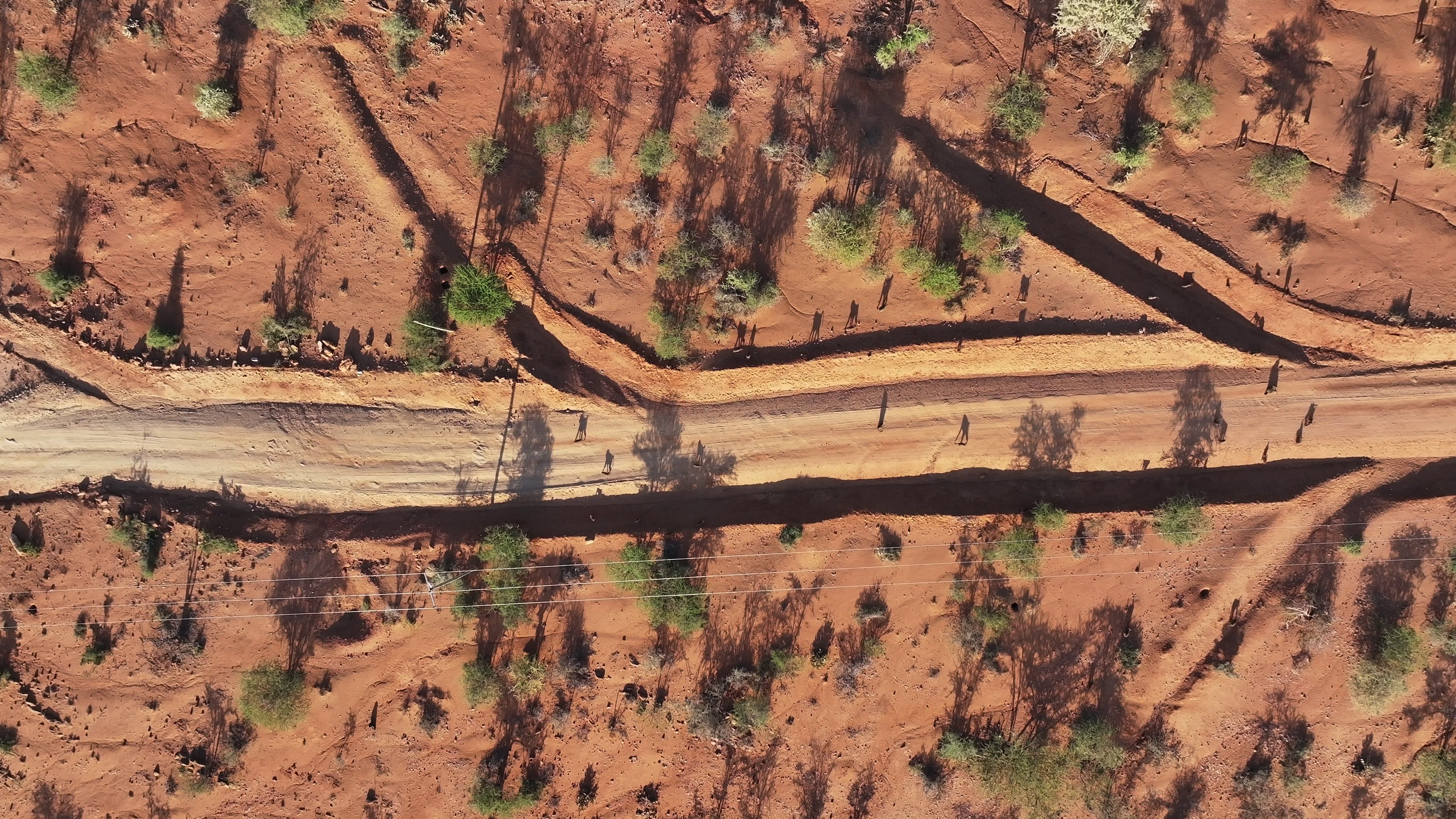
One of my first tasks was to collect representative footage to understand what the data actually looks like “in the wild,” including terrain, lighting, motion blur, and compression artifacts. I wasn’t able to travel to Kenya, but we had a lucky alignment: the BBC was filming a documentary with the UNBP team. I coordinated capture requirements for drone filming (altitude, camera angle, overlap, stabilization settings when possible), and they returned several hours of high-quality aerial video across multiple environments and lighting conditions.
Fun fact: the documentary is called "The Secret Life of Animals" on Apple TV+. Episode 10 features the baboons we studied, and a split-second of our aerial footage appears in that segment.
Next, I organized annotation sessions with E4E volunteers using Label Studio. We labeled several thousand frames with bounding boxes around each baboon. This became the Laikipia Baboon Aerial Dataset (LBAD).
To avoid overfitting to one domain, we also adopted an “agnostic” benchmark dataset. Our goal was not “baboon-only” tracking; we wanted a pipeline that generalizes to small-object multi-target tracking in aerial video. Satellite highway traffic footage has similar characteristics (high viewing angle, small objects, weak appearance cues), so we used the Video Satellite Object (VISO) dataset. VISO also provides published baselines, which gave us a strong comparison point.
Algorithm Development
The algorithm we developed—Spot—was primarily the work of the master’s student I assisted as part of his thesis. The thesis is available here, and the code is open-sourced on GitHub.
Spot targets the “hard mode” of aerial tracking: small, low-contrast objects (sometimes as small as ~30×30 px) in video with non-stationary camera motion and camera-induced pseudo-motion. At a high level, it:
- Aligns historical frames into the current frame’s coordinate space (to compensate camera motion),
- Extracts motion to produce candidate foreground regions,
- Links regions over time, using temporal filtering (particle-filter style tracking) to stabilize tracks.
Evaluation
To evaluate Spot, we also needed strong baselines. We selected several methods reported as competitive on VISO, including ClusterNet, D&T, AGMM, and MMB. Two of these (AGMM and MMB) did not have usable public implementations for our needs, so I reimplemented them from the papers.
Baseline 1: AGMM (C++ / OpenCV)
AGMM is a classic background subtraction approach where each pixel is modeled by an adaptive Gaussian mixture model (GMM). I implemented AGMM in C++ (OpenCV-based), and intentionally designed it with a clean object model because AGMM naturally decomposes into nested parts:
AGMM(video-level orchestrator: per-frame update + mask production)Mixture(per-pixel mixture model with update rules, match/replacement logic, and eta scheduling)Gaussian(mean / variance / weight container)
This modular structure made it easier to:
- debug per-pixel behavior,
- inspect learning-rate evolution (
eta) over time, - parallelize the per-pixel update loop (optional OpenMP),
- and later integrate visualization tools without rewiring the math.
What the AGMM pipeline produced
For each frame, the implementation generated three masks:
- Object mask (foreground candidates)
- Shadow mask (optional suppression pass)
- Final mask = object mask − shadow mask
And then produced a “result image” by applying the final mask to the input frame:
this->backgroundModelMaintenance();
this->foregroundPixelIdentification();
if (!this->disableShadow) this->shadowDetection();
this->finalMask = this->objectMask - this->shadowMask;
this->objectExtraction();
this->objectTypeClassification();
cv::bitwise_and(this->frame, this->frame, this->result, this->finalMask);
The GitHub repo can be found here.
Baseline 2: MMB (MATLAB)
For MMB, the algorithm is organized into three modules:
- AMFD — Accumulative Multi-Frame Difference
- LRMC — Low-Rank Matrix Completion (foreground via low-rank + sparse decomposition)
- PF — Pipeline Filter (temporal consistency filter + lightweight association)
Because MMB’s LRMC stage closely follows fRMC, which already had a public MATLAB implementation, it was practical to implement the full MMB pipeline in MATLAB to reduce friction and keep everything in one environment.
What I implemented and added beyond “straight porting”
1. A robust, configurable CLI-style entry point (baboon_mmb)
I implemented baboon_mmb.m as a single function that:
- validates parameters (ranges + cross-constraints like AREA_MIN ≤ AREA_MAX),
- loads an image sequence,
- runs AMFD + LRMC,
- combines masks via AND/OR,
- runs PF to emit bounding boxes,
- and optionally saves intermediate artifacts.
This turned MMB into a reproducible tool rather than a notebook-only prototype.
objects = baboon_mmb('IMAGE_SEQUENCE', 'path/to/frames', 'FRAME_RATE', 10, ...
                    'K', 4, 'AREA_MIN', 5, 'AREA_MAX', 80, ...
                    'PIPELINE_LENGTH', 5, 'H', 3, ...
                    'DEBUG', true);
2) Deterministic output artifacts for inspection
When DEBUG=true, the pipeline writes:
- masks for each stage (
output/amfd,output/lrmc,output/combined) .matdumps of masksobjects.matandobjects.txt- bounding-box visualizations in
output/frames
That made it easy to compare failure cases and isolate whether AMFD, LRMC, or PF was responsible.
3) Parallel LRMC option
LRMC is often the bottleneck. I added a parallel option (USE_PARALLEL_LRMC, NUM_WORKERS) that:
- respawns the MATLAB pool cleanly,
- splits the frame range into chunks,
- runs
processFrame()per worker, - and merges outputs deterministically.
lrmcMasks = lrmc(args.L, args.KERNEL, args.MAX_NITER_PARAM, ...
                 args.GAMMA1_PARAM, args.GAMMA2_PARAM, args.FRAME_RATE, ...
                 grayFrames, args.USE_PARALLEL_LRMC, args.NUM_WORKERS);
4) PF: a practical temporal consistency filter
MMB’s published method included a PF stage but did not ship a turnkey tracker. I implemented PF as a temporal filter that:
- buffers masks across
PIPELINE_LENGTH, - performs assignment using
matchpairswith Euclidean distance costs, - only emits objects that appear consistently in at least
Hof buffered frames, - and optionally interpolates missing detections to keep tracks stable.
objects = pf(args.PIPELINE_LENGTH, args.PIPELINE_SIZE, args.H, combinedMasks);
This PF stage was crucial for reducing one-frame “sparkle” detections that are common in aerial and satellite video.
The GitHub repo can be found here.
Experimental Setup
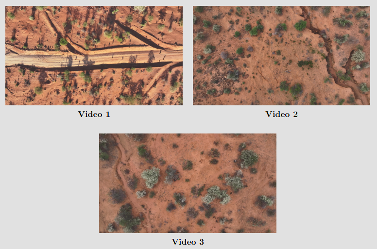
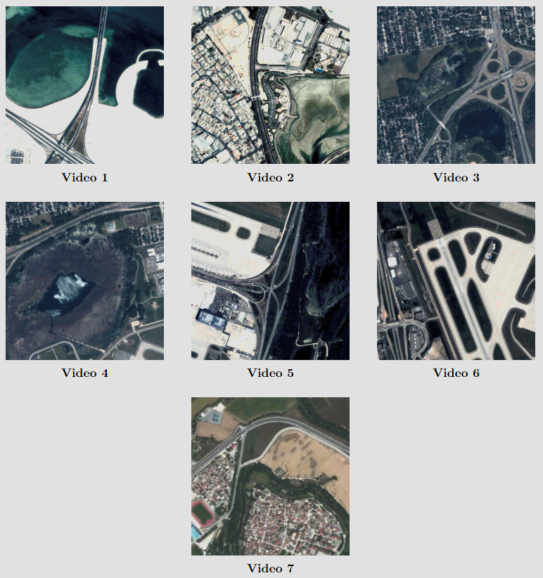
Due to budget constraints, we evaluated Spot against MMB on:
- 7 VISO videos (a subset used in the original VISO paper for MMB evaluation)
- 3 LBAD videos
We chose MMB because it was among the strongest reported baselines on VISO, and we wanted a hard comparison against a method already competitive on the benchmark.
Since MMB did not include a full tracking pipeline comparable to Spot’s identity maintenance, we evaluated detection performance using:
- Precision
- Recall
- F1-score
- AP / mAP
We ran sweeps over hyperparameters and configurations on AWS EC2 over several months.
Results
The tables below summarize detection performance on LBAD and VISO.
LBAD
| Video | Algorithm | Precision | Recall | F1 | AP |
|---|---|---|---|---|---|
| 01 | MMB | 0.6511 | 0.4983 | 0.5645 | 0.5361 |
| 01 | Spot | 0.6062 | 0.4658 | 0.5268 | 0.5362 |
| 02 | MMB | 0.5943 | 0.5072 | 0.5473 | 0.5111 |
| 02 | Spot | 0.7534 | 0.6530 | 0.6996 | 0.7018 |
| 03 | MMB | 0.5110 | 0.6257 | 0.5626 | 0.5145 |
| 03 | Spot | 0.6022 | 0.8046 | 0.6888 | 0.6977 |
Overall mAP: 0.521 (MMB) vs 0.645 (Spot)
VISO
| Video | Algorithm | Precision | Recall | F1 | AP |
|---|---|---|---|---|---|
| 01 | MMB | 0.7378 | 0.8203 | 0.7769 | 0.7949 |
| 01 | Spot | 0.3601 | 0.3796 | 0.3696 | 0.2583 |
| 02 | MMB | 0.6933 | 0.5971 | 0.6416 | 0.6867 |
| 02 | Spot | 0.6442 | 0.6167 | 0.6301 | 0.6744 |
| 03 | MMB | 0.7417 | 0.8117 | 0.7751 | 0.7414 |
| 03 | Spot | 0.5477 | 0.7074 | 0.6174 | 0.5795 |
| 04 | MMB | 0.7248 | 0.5945 | 0.6532 | 0.6611 |
| 04 | Spot | 0.7119 | 0.6482 | 0.6786 | 0.6508 |
| 05 | MMB | 0.7640 | 0.7218 | 0.7423 | 0.7156 |
| 05 | Spot | 0.6457 | 0.6329 | 0.6393 | 0.6212 |
| 06 | MMB | 0.6993 | 0.6953 | 0.6973 | 0.7186 |
| 06 | Spot | 0.7358 | 0.6323 | 0.6802 | 0.7210 |
| 07 | MMB | 0.7757 | 0.6706 | 0.7193 | 0.7161 |
| 07 | Spot | 0.9337 | 0.5481 | 0.6907 | 0.7440 |
Overall mAP: 0.719 (MMB) vs 0.607 (Spot)
Discussion
Patterns across datasets
On LBAD, Spot achieves higher overall mAP than MMB and leads on two of three videos (Videos 02–03). The contradiction between LBAD Video 01 and Videos 02–03 is likely explained by the substantially lower individual count in Video 01. When both algorithms are tuned to compensate for very few instances, they tend to over-detect pseudo-motion relative to the individuals of interest. In Videos 02 and 03, where the individual count is moderate to abundant, Spot performs higher on both precision and recall, indicating stronger detection when more agents are present.
On VISO, MMB attains higher overall mAP than Spot, although the scores remain close. A main contributor to Spot’s lower AP is VISO Video 01, which contains mostly bay water; under compression this produces sharp contrast variations (more than a higher-resolution pond would), violating Spot’s assumption of a mostly static background. Outside these edge cases, Spot is comparable to strong baselines in satellite-video multi-object detection, suggesting it is not overfit to a single domain.
Implications and limitations
While both algorithms—especially Spot—show positive results on LBAD, neither alone fully satisfies the needs of robust multi-agent tracking at high drone altitudes. Spot detects moving individuals well, but its ability to maintain identities and detect individuals that are momentarily stationary is not fully benchmarked. It should be viewed as a strong baseline to iterate on, rather than a complete, foolproof pipeline.
Compute resources and time are additional constraints in real-world field settings. In many studies, researchers may only have access to a basic laptop (sometimes without a discrete GPU) or a modest desktop. Spot and MMB can take over an hour to process a single video and may require more than 64 GB of memory.
That said, with further optimization—and in some cases trading accuracy for speed—these methods can still be valuable as a first pass in labeling workflows. Model-assisted annotation systems (e.g., CVAT, Label Studio, VIAME/DIVE) can accept pre-labels from detectors or motion models, propagate tracks, and support human correction inside a UI. A practical workflow for LBAD-like studies is to generate proposals with a motion-first method such as Spot, and then have an annotator refine labels efficiently.